Week 6: Analyzing proportions
Wed, Mar 7, 2018 Made by Judit Kisistók. Supplemented by Simon Grund Sørensen. The exercise session was created by Thomas Bataillon and Palle Villesen at Aarhus University.library(tidyverse) # I will need this later for fancy plottingLearning goals
By the end of this session, you should be able to…
- understand several key concepts within hypothesis testing:
- null hypothesis & null distribution
- test statistic & P-values
- which errors can we make when performing hypothesis testing (I and II)
- what is statistical power
- understand the binomial distribution and in what context it arises
- how the binomial probability distribution can be used as a null distribution when testing null hypothesis with proportion data
README FIRST :-)
We first introduce/illustrate two important new R functions: dbinom() and rbinom(). You then have to reuse these 2 functions in a variety of situations.
It’s a good idea to work sequentially:
1. Try the R function and how they relate to the binomial distribution of Chapter 7 and how to graph the distribution
2. Try the next questions that basically redo in R some examples of Chapter 7
3. Try the set of Chapter 7 problems
4. Try the last question on statistical power (more challenging)
Introducing dbinom() and rbinom()
R functions for simulating from /calculating the binomial probability
If you want to draw 1 random number from a binomial distribution with 25 trials(tests) and probability of success 1/2
rbinom(n = 1, size = 25, prob = 0.5) ## try to evaluate that several times (you get different numbers)## [1] 12If you want to calculate the probability of having exactly 2 success out of 25 trials
dbinom(x = 2, size = 25, prob = 0.5)## [1] 8.940697e-06Using dbinom() and rbinom()
Let’s call X3 the random variable that records the number of “6” you get when rolling 3 dices. Use rbinom() and generate 100 observations from X3 (instead of just 1 observation).
rbinom(n = 100, size = 3, prob = 1/6)## [1] 0 1 0 0 1 0 1 2 0 1 0 1 1 0 0 1 1 1 1 0 1 1 1 0 0 1 0 0 0 0 2 0 2 0 1
## [36] 1 1 0 2 0 0 2 0 0 1 0 1 0 1 0 0 0 0 0 0 0 0 1 0 0 1 1 1 0 0 0 1 0 0 0
## [71] 2 1 1 0 0 0 0 1 0 1 1 1 0 1 1 0 0 2 1 0 0 2 0 0 1 1 0 0 1 0# we want 100 observations
# we have 3 dice - so the number of trials is 3
# and the probability of getting a 3 is 1/6Using dbinom(), Calculate P(X3=0) and P(X3 = 2).
dbinom(x = 0, size = 3, prob = 1/6)## [1] 0.5787037dbinom(x = 2, size = 3, prob = 1/6)## [1] 0.06944444Take me back to the beginning!
Visualizing the binomial distribution in R
We can simulate 1000 times from the binomial and make a histogram like in example 7.1-1
nleftHanded= rbinom(n = 10^3, size =27, p=0.25) # Simulated H0 distribution for the number of left handed flowers

hist(nleftHanded, prob=T, breaks=seq(from=0, to = 27, by = 1), col="deeppink4",
     xlab="Number of lefthanded flowers (X)",
     ylim=c(0,0.2),
     ylab="Probability")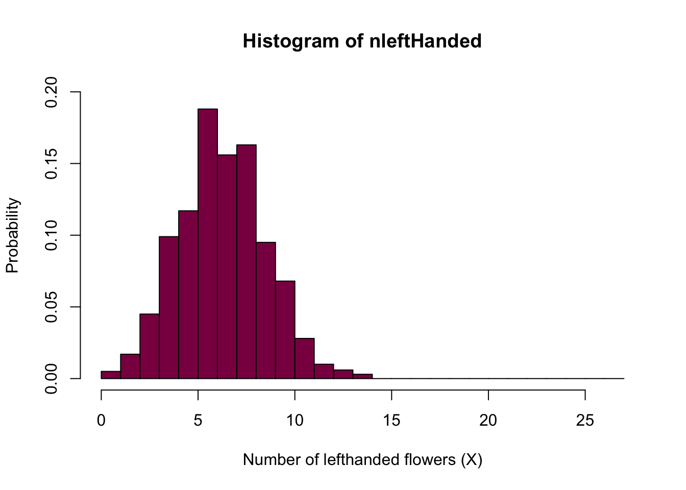
We can also directly get the exact probability from the binomial distribution:
nLeftFlowers=seq(from=0, to = 27, by = 1) #creates a sequence of numbers from 0 to 27 - you can think about this as "bins" on your histogram
PnL=dbinom(x = nLeftFlowers, size = 27, prob = 0.25 ) # exact H0 distribution for the number of left handed flowers - we take the sequence of numbers ("bins") we created before and calculate the probabilities for every single one (aka the probability of observing 0, 1, 2...27 left-handed flowers out of 27 if the probability of being left-handed is 0.25)

sum(PnL) # sanity check (if it is a probability --> sums to 1)
## [1] 1plot(nLeftFlowers,PnL, type ="h", col="deeppink4", lwd=5) #lwd is just the width of the lines, so you can play around with it and see if you find a different line width more aesthetically pleasing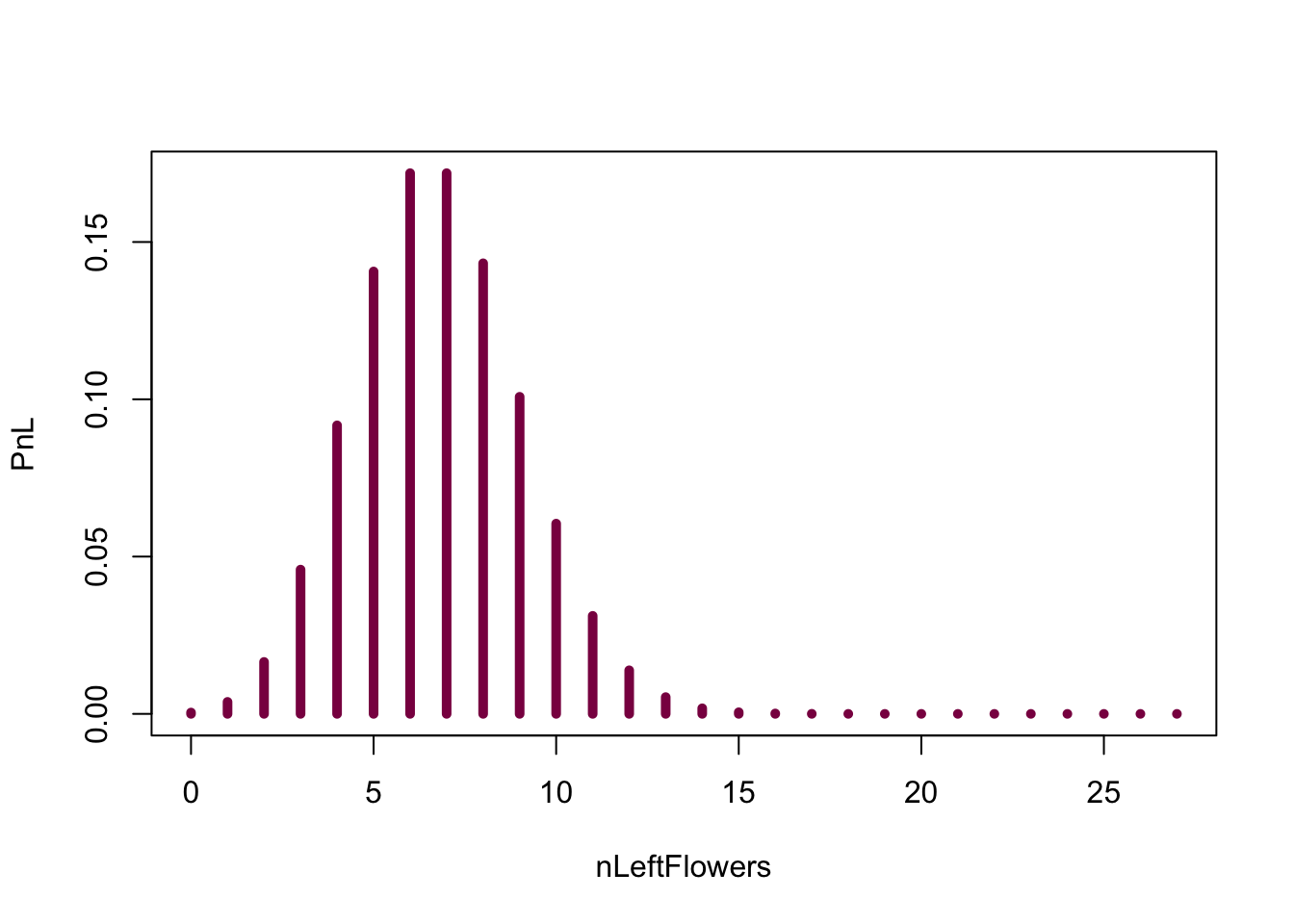
Take me back to the beginning!
Example 7.2 of the book “Sex and the X” in R
Let’s just recap briefly: out of 25 spermatogenesis genes, 10 are located on the X (that makes up 6.1 % of the mouse genome).
And the biological question is: How improbable is this, if the X gene reportoire was not special? The H0 (p. 186) is that the probability of any spermatognesis gene falls on X is 6.1%.
Graph the (null) probability distribution for SunderXh0, the number of spermatogenesis genes that are on the X under H0.
# Simulated
SunderXh0 = rbinom(n = 10^3, size = 25, p=0.061) # simulated nulldistribution for the number of spermatogenesis genes falling on X under H0 - we have 25 genes in total and the probability of falling on the X is 0.061 under the null
# what rbinom does is that it gives you a bunch (10^3) random numbers from the binomial distribution - and depending on the probability, you may or may not see every possibility / event happening

hist(SunderXh0, prob=T, breaks=seq(from=0, to = 27, by = 1), col="deeppink4",
     xlab="Number of genes on Chromosome X given H0",
     ylim=c(0,0.2),
     ylab="Probability",
     main = "Simulated H0 distribution from 1000 simulations")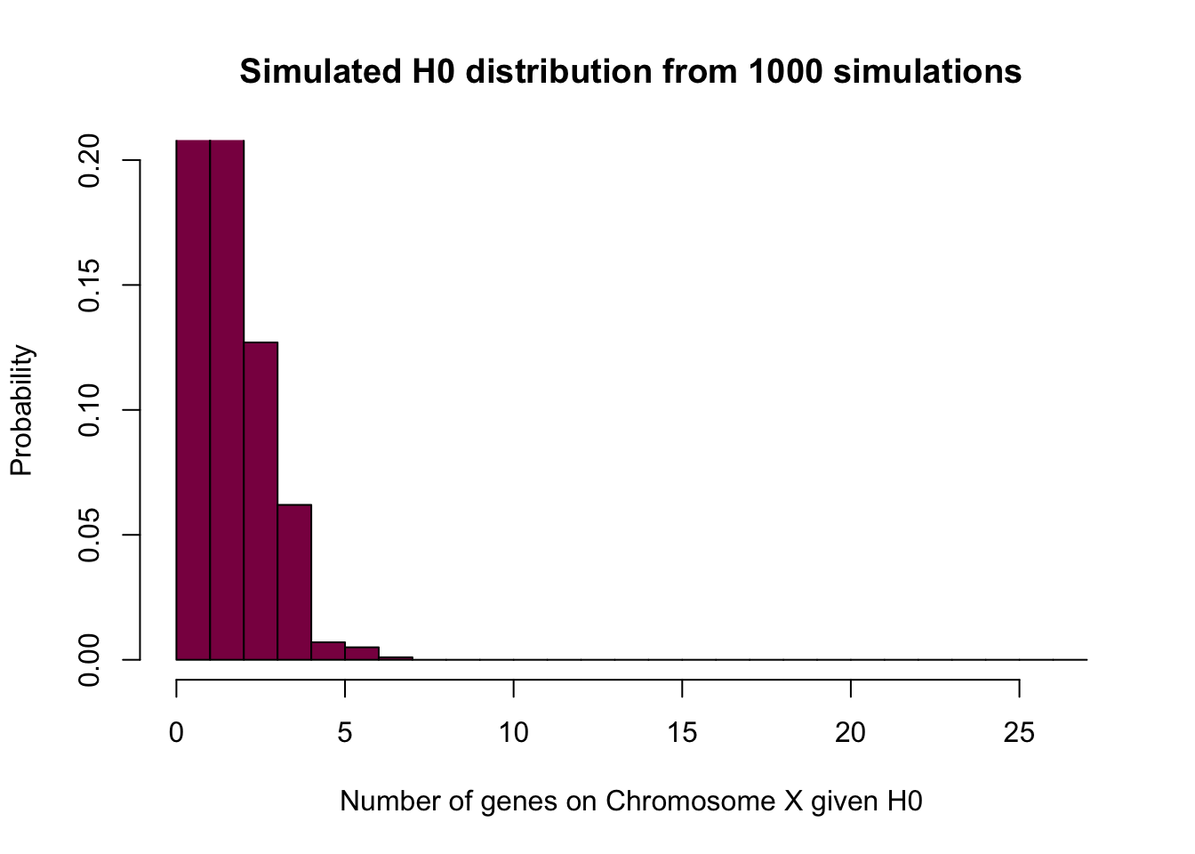
# here you can see that there is not much to look at after X = 7 - the probability of observing more is so small that 1000 simulations are not enough to observe them at least once

# Exact
SunderXh0=seq(from=0, to = 25, by = 1)
Pr_sunderXh0=dbinom(x = SunderXh0, size = 25, prob = 0.061) # exact H0 distribution for the number of spermatogenesis genes falling on X under H0

# this one is exact because you are not relying on your luck (and simulation) and hope that you'll observe every possibility at least once - instead, you are calculating the exact probabilities of observing 0, 1...25 genes on the X under H0

sum(Pr_sunderXh0) # sanity check (if it is a probability --> sums to 1)
## [1] 1plot(x = SunderXh0, y = Pr_sunderXh0, type ="h", col="deeppink4", lwd=7, main = "Exact H0 distribution") 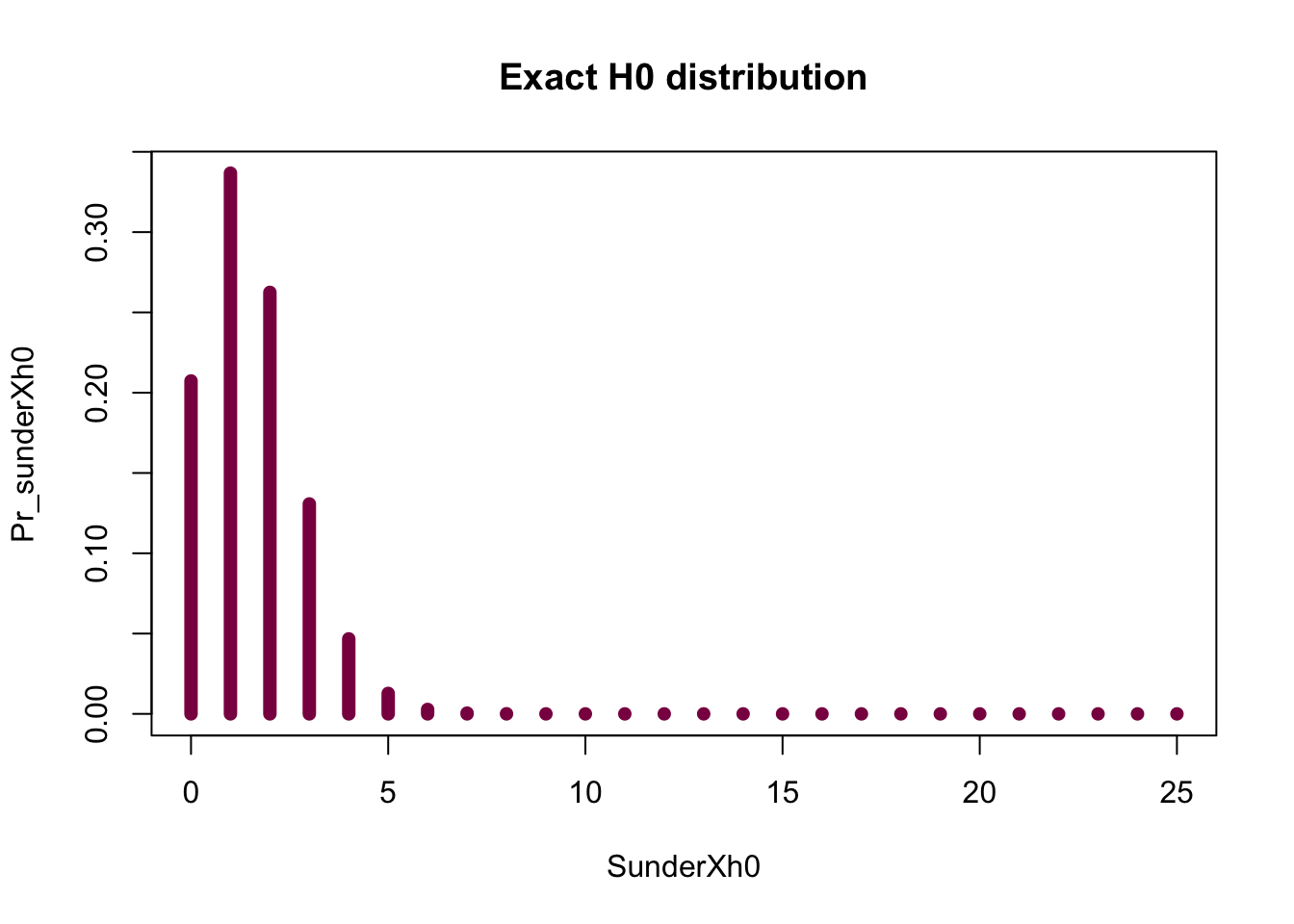
Calculate Pr(SunderXh0 > 10).
#Sum the probabilities from being 11 and above
sum(Pr_sunderXh0[11:25])
## [1] 9.93988e-07Why is the p value for this case calculated as 2* Pr(SunderXh0 > 10)?
Because we reject the null hypothesis in two cases - if there are more spermatogenesis genes on X than expected under the null, or if there are less, hence, we’re looking at a two-tailed test. To get the P-value, we need to take into account both extremes - the probability that we see 10 or more spermatogenesis genes on the X and its equivalent in the lower tail.
It is not immediately apparent what the “equivalent lower tail” is in this case because the distribution is asymmetrical - however, you can think about it in terms of probabilities. If you sum up the probability from being 11 and above, you get a value y - and in the lower tail, you will find the same y probability and that is going to be your equivalently extreme lower tail. However, note that it is not always so - the analysis always depends on the data and the questions you’re asking!
If you are unsure whether you should multiply by 2 to get the P-value, think about the null hypothesis. If it’s like this:
\(H_0: p_0 = 0.5\) - the opposite of this is:
\(H_A: p_0 =/= 0.5\).
This means that you need to look at both extremes. On the other hand, if the null hypothesis looks like this:
\(H_0: p_0 >= 0.5\) - the corresponding alternative hypothesis is this:
\(H_A: p_0 < 0.5\), in which case you are only interested in one extreme.
Simulation based p-value versus exact p-values
Using 10^5 simulations, simulate the null distribution for SunderXh0 and get the (approximate) p-value by comparing the simulated distribution and the data.
SimulatedP= rbinom(n = 10^5, size =25, p=0.061) # Simulated H0 distribution for the number of left handed flowers

2*(sum(SimulatedP>10)/(10^5)) #P-value of 10 or more genes on X, assuming H0 - you sum up the simulated values that are larger than 10, divide it by the total number of simulations and multiply it by 2 to get the P-value for this two-tailed test
## [1] 0Why are the exact p-value and the approximate p-value you got different? (Hint: think about how many simulations you need to do in order to observe an event that has probability 0.0001 versus 0.0000001?).
If an event has a very small probability, we need to do a huge amount of simulations to be able to observe it at least once - so these events might get lost when we’re doing simulations to determine the p-value, but are covered in the exact p-value calculations.
Take me back to the beginning!
Chapter 7 Problems
Answers to problems 1, 2, 5, 6, 13 and 16 can be found in the book.
Exercise 24
- On average, 0.25 of 12 peas should be wrinkled - which is 3.
0.25*12## [1] 3- The standard error of an estimate is the standard deviation of the sampling distribution - in this case, the standard error of the proportion estimate.
n = 12
prop_estimate = 0.25 #expected fraction of wrinkled peas
SE = sqrt((prop_estimate*(1-prop_estimate))/n)
SE
## [1] 0.125- The variance is the square of the standard deviation.
var = SE**2
var
## [1] 0.015625- The proportion of students seeing exactly 2 wrinkled pea plants:
dbinom(x = 2, size = 12, prob = 0.25)## [1] 0.2322932Take me back to the beginning!
Planning a survey according to statistical power
Imagine that you are planning a survey where you want to show that a species has a biased sex ratio. The null hypothesis is that the ratio is balanced (1/2 males and 1/2 females at birth), but you suspect that the sex ratio in that species is actually 1/3 2/3.
What mimimum number of individuals should you examine (i.e. sex determine) in order to have have a power of 90% to reject the null (we use a type I error of 0.01 to reject the null)?
First of all, pick a sample size and see if you can simulate the null and the alternative distributions (remember that we have a specific alternative hypothesis so this should be doable). Plot them and see how far they are from eachother - if there is a huge overlap, that implies that you don’t have enough power to reject the null at that sample size.
What we want is really just the following - finding a sample size where 99.5% of the \(H_0\) distribution is above the lower tail significance threshold and 90% of the \(H_A\) distribution is below that threshold.
We need to set the 99% significance threshold on the \(H_0\) distribution and then calculate how many \(H_A\) values are lower than this - this number is going to be the power.
So, in a nutshell:
- Figure out the null you want to reject and the critical value at 0.01 levels
- Simulate different null distribution until you have 90% of the simulated value that reject the NULL
Here is one solution. Let’s pretend that someone told us that n = 120, but feel free to play around with it and see what happens if it’s way less.
xs=seq(from =0, to =120, by=1)
H0=dbinom(x = xs,size = 120,prob = 0.5) #the null distribution
HA = dbinom(x = xs,size = 120,prob = 2/3) #the alternative distribution
data = as.data.frame(cbind(xs, H0, HA)) #putting everything to one dataframe for convenience

# What's the treshold where 90% of data is expected to lie within?
i = seq(1,120,1) # just numbers from 1 to 120
p = 2 * (1-pbinom(q = i,size = 120,prob = 0.5)) # 120 p-values
treshold = as.data.frame(cbind(i, p))

# let's plot it - the horizontal line signifies that threshold:
ggplot(treshold)+
  geom_point(aes(i,p))+
  geom_hline(aes(yintercept = 0.1))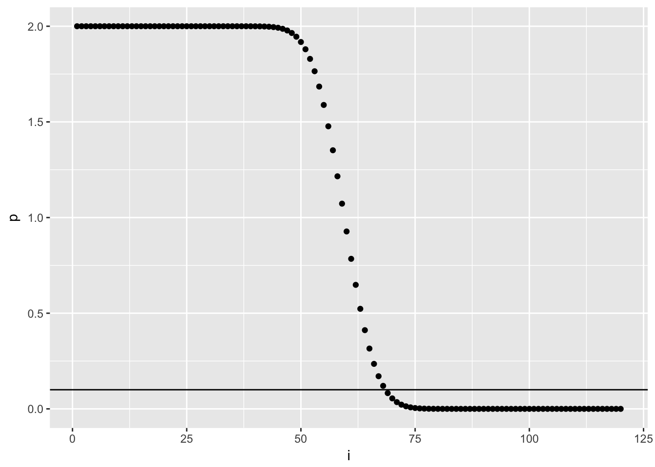
# another plot to show the distributions
ggplot(data)+
geom_histogram(aes(x = xs, y = H0, fill = "H0"), stat = "identity", alpha = 0.80)+
geom_histogram(aes(x = xs, y = HA, fill = "HA"), stat = "identity", alpha = 0.60)+
ylab("")+
geom_vline(aes(xintercept = 72))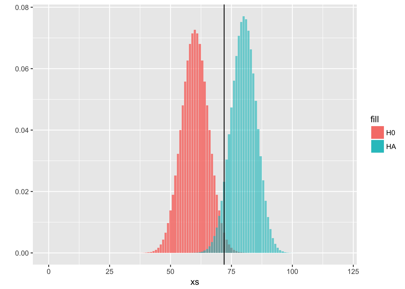
# we measure how many values from HA are over this threshold, which is going to be our desired power
cat("Power, with n = 120 and significance level = 0.1:" ,1-pbinom(q = 72,size = 120,prob = 2/3))
## Power, with n = 120 and significance level = 0.1: 0.9253669Let’s see another solution with classic plots and less steps.
Here you know that \(H_A\) is binomial wih n trials and p = 2/3 and you can only vary n. Here is an approx answer that gives about 90% power (actually 85%) with n=120:
xs=seq(from =0, to =120, by=1)
MypH0=dbinom(x = xs, size = 120, prob = 0.5)
# calculate the number of individuals that would result in NOT rejecting the null and the number of individuals that would result in rejecting the null - this is the threshold we're looking for, which is 74 individuals in this case
1-pbinom(q = 74,size = 120,prob = 0.5)
## [1] 0.003923297MypHA=dbinom(x = xs,size = 120,prob = 2/3)
plot(xs,MypH0, col="black", type="h", lwd=3, xlab="xs", ylim=c(0,0.1), ylab="Probability", cex.axis=1.6)
abline(v=74, col="red", lwd=2, lty=2)
points(xs+0.2,MypHA, col=" green", type="h", lwd=3)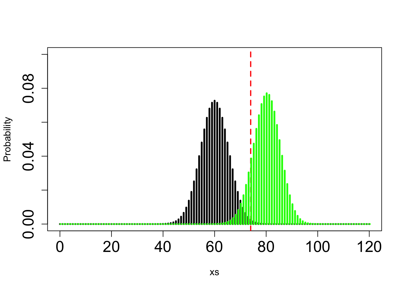
1- pbinom(q = 74, prob = 2/3,size = 120) #the power## [1] 0.8563232Take me back to the beginning!